Root-Locus Method

6.1 Basic root-locus construction

e.g. 6.1.1

\[C(s)=K_p, \quad P(s) = \frac{1}{s(s+2)}\]
\[\begin{align} \pi(s) &= s^2 + 2s + K_p\\ s &= -1 \pm \sqrt{1-K_p}\\ \end{align}\]

• If \(K_p \le 0\), lose IO stability
• If \(0 \lt K_p \le 1\), we have two roots with negative real part

• This root locus tells us that the system can go unstable with bad choices of \(K_p\)
• From the diagram, we can qualitatively see that \(K_p\) should be such that \(\Im(s)\) of the poles \(\ne 0\), but not too big.
• Matlab: use sisotool or rltool

Construction

\[\pi(s) = \underbrace{D_pD_c}_{D(s)} + K\underbrace{N_pN_c}_{N(s)}\]

A root-locus diagram is a drawing of how the roots of \(\pi\) change as \(K\) is changed.

Assumptions:

• \(C(s)P(s)\) proper
• \(K \ge 0\)
• \(D(s)\) and \(N(s)\) are monic (leading coefficient is 1)

Let \(n:=\deg(D(s))\), \(m:=\deg(N(s))\)

Rules

1. Roots of \(\pi\) are symmetric about the real axis
2. There are \(n\) "branches" (paths) of the root locus (since \(\deg(\pi)=n\))
3. Roots of \(\pi\) are a continuous function of \(K\)
4. When \(K=0\), roots of \(\pi\) are equal to the roots of \(D\)
5. As \(K \rightarrow +\infty\), \(m\) branches of the root locus approach the roots of \(N(s)\) (\(\pi(s) = 0 \Leftrightarrow \frac{N(s)}{D(s)}=\frac{-1}{K}\))
6. The remaining \(n-m\) branches tend towards \(\infty\). They do so along asymptotes:
   • Go through the point \(s=\sigma + 0j\) where \(\sigma = \frac{\sum \text{roots of } D - \sum \text{roots of } N}{n-m}\) (centroid)
   • Make angles \(\phi_1, ...,\phi_{n-m}\) with real axis given by \(\phi_k := \frac{(2k-1)\pi}{n-m}, k \in \{1, ..., n-m\}\)
   • Asymptote patterns: (fig. 6.4)
   • 
7. ("no-yes-no" rule) A point \(s_0\) on the real axis is a part of the root locus if and only if \(s_0\) is to the left of an odd number of poles/zeroes.
   • It follows from the fact that on the root locus, \(\angle N(s_0) - \angle D(s_0) = \angle \frac{-1}{K} = \pi\)
8. (angles of departure/arrival)
   • 
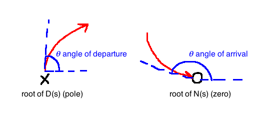
   • To compute, use \(\angle N(s) - \angle D(s) = \pi\)
   • \(\Rightarrow \angle (s-z_1) + \angle (s-z_2) + ... + \angle(s - z_m) - \angle (s-p_1) + ... + \angle (s-p_n) = \pi\)
   • To compute the angle of departure at pole \(p_i\), plug \(s=p_i\) into the above and solve for \(\angle (s-p_i) =: \theta_{p_i}\).

Procedure for plotting root-locus

Given an \(n\)th-order polynomial \(\pi(s)=D(s)+KN(s)\)

1. Compute the roots \(\{z_1, ..., z_n\}\) of \(N(s)\) and place a circle at each location.
2. Compute the roots \(\{p_1, ..., p_n\}\) of \(D(s)\) and place an X at each location.
3. Use rule 7 ("no-yes-no") to fill in the real axis
4. Compute centroid \(\sigma\), label the point \(s=\sigma +j0\) in \(\mathbb{C}\)
5. Compute and draw the \(n-m\) asymptotes
6. Compute angles using rule 8. Usually only needed for complex conjugate rots and repeated real roots.
7. Give a reasonable guess of how it looks (symmetric around real axis!)

e.g. 6.3.1

\[P(s)=\frac{1}{s^2+2s+5}, \quad C(s)=K\left(1+\frac{1}{0.25s}\right)\]

\[\begin{align} \pi(s)&=N_cN_p+D_cD_p\\ &= s(s^2+2s+s)+K(s+4)\\ &=:D(s)+KN(s)\\ \end{align}\]

1. \(N(s)=s+4 \Rightarrow z_1=-4, m=1\)
2. \(D(s)=s(s^2+2s+s) \Rightarrow n=3, \{p_1, p_2, p_3\}=\{0, -1+2j, -2-2j\}\)
3. "no-yes-no"
4. \(\sigma = \frac{0+(-1+2j)+(-1-2j)-(-4)}{3-1}=1\)
5. \(n-m=2 \Rightarrow \phi_1=\frac{\pi}{2}, \phi_2=\frac{-\pi}{2}\)
6. Compute departure angle for \(p_2\) (no need for \(p_3\), we know it from symmetry):
   • \(\pi(s)=D(s)+kN(s)=0 \Leftrightarrow \frac{N(s)}{D(s)}=\frac{-1}{K}\)
   • \(\angle N(s) - \angle D(s) = \pi\)
   • \(\angle(s+4)-\angle s - \underbrace{\angle(s+1-2j)}_{\theta_{p_2}}-\angle(s+1+2j) = \pi\)
   • \(\theta_{p_2} = \angle (p_2+4) - \angle p_2 - \angle (p_2 + 1 + 2j) - \pi\)
   • \(\theta_{p_2} = \angle(-3+2j)-\angle(-1+2j)-\angle 4j - \pi\)
   • \(\theta_{p_2} = 7.125^\circ\)

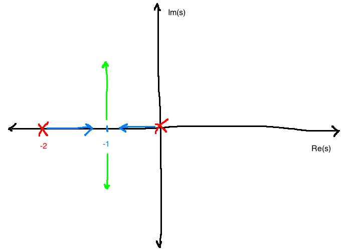
e.g. 6.2.2

\[\pi(s)=D(s)+KN(s), \quad D(s)=s^3(s+4), \quad N(s)=s+1\]
\(n=4\)
\(m=1\)

\(\sigma = \frac{-4 - (-1)}{4-1} = -1\)

e.g. Cart pendulum system

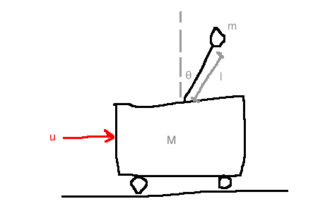
\[\frac{Y(s)}{U(s)} = P(s)=\frac{\frac{1}{Ml}}{s^2 - \frac{g}{Ml}(m+M)}\]

6.2.3 Proportional controller

Try \(C(s)=K_p\). We get:
\[\begin{align} \pi(s)&=D_pD_c+N_pN_c\\ &=s^2-\frac{g(M+m)}{Ml}+\frac{K_p}{Ml}\\ \\ D(s)&:=s^2-\frac{g}{Ml}(m+M)\\ N(s)&:=1\\ K&:=\frac{K_p}{Ml}\\ \end{align}\]

Asymptotes: \(\sigma = 0\)
\(n-m=2-0=2\)

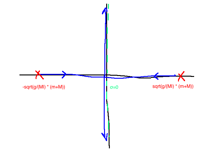
Proportional control won't work.

Matlab: suppose you have a controller \(P(s)C(s)=\frac{8(s+2)}{(s+1)(s+5)(s+10)}\). In matlab:

z = -2;
p = [-1 -5 -10];
k = 8;
L = zpk(z, p, k) % Zeroes, Poles, gain
rlocus(L);

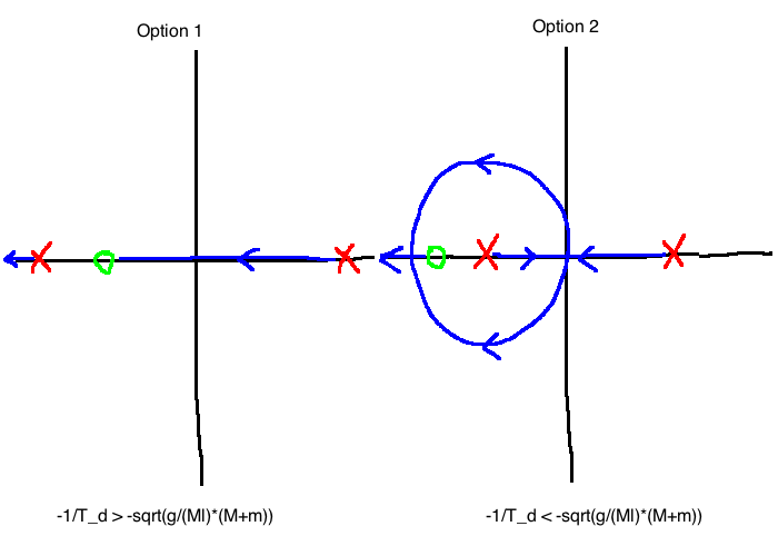
6.2.4 P.D. Control

\[\begin{align} C(s) &= K_p(1+T_ds)\\ &= K_pT_d\left(s+\frac{1}{T_d}\right)\\ \\ \pi(s) &= \underbrace{s^2- \frac{g}{Ml}(M+m)}_{D(s), \quad n=2} + \underbrace{\frac{K_pT_d}{Ml}}_{K}\underbrace{\left(s+\frac{1}{T_d}\right)}_{N(s), \quad m=1}\\ \end{align}\]

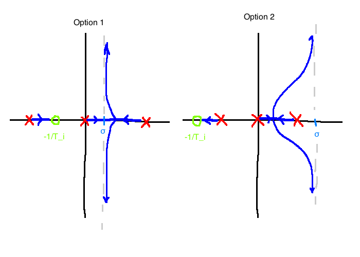
6.2.5 P.I. Control

\[\begin{align} C(s)&=K_p\left(1+\frac{1}{T_is}\right)\\ &= K_p \frac{s+\frac{1}{T_i}}{s}\\ \\ \pi(s) &= \underbrace{s\left(s^2-\frac{g}{Ml}(m+M)\right)}_{D(s)} + \underbrace{\frac{K_p}{M_l}}_K \underbrace{\left(s+\frac{1}{T_i}\right)}_{N(s)}\\ \\ \sigma &= \frac{1}{2T_i}\\ \end{align}\]

6.3 Non-standard problems

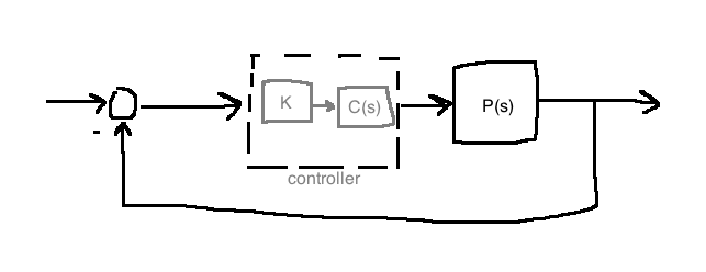
Non-unity feedback

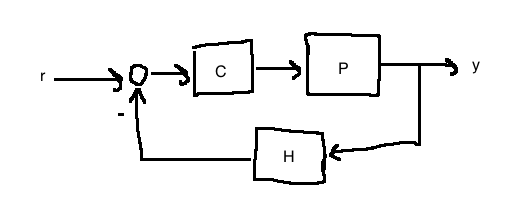
In this case, the characteristic polynomial is:
\[\pi(s)=N_pN_cN_h + D_pD_cD_h\]

Identify \(D\), \(N\), and \(K\), and proceed as before.

Controller isn't a linear function of the gain

Even if we can't factor \(K\) out from \(C(s)\), the characteristic polynomial can still be expressed in the form \(\pi(s)=D(s)+KN(s)\), but now, \(D \ne D_pD_c\) and \(N \ne N_pN_c\)

e.g.

\[\begin{align} P(s)&=\frac{1}{s(s+2)}\\ C(s) &= 10(1+T_ds)\\ \\ \pi(s)=D_pD_c+N_pN_c\\ &= \underbrace{s^2+2s+10}_{D(s)} + \underbrace{10T_d}_K \underbrace{s}_N\\ \\ \text{Observe:}\\ D(s)=s^2+2s+10 \ne D_pD_c\\ N(s)=s \ne N_pN_c\\ \end{align}\]

Then proceed as before.

Improper Loop Gain

\[\pi(s)=D(s)+KN(s)\]
Normally, \(\deg(D) \ge \deg(N)\). In this case, we have the opposite: \(\deg(D) \lt \deg(N)\).

\[\pi(s) = 0 \Leftrightarrow N(s) + \frac{1}{K}D(s)=0\]

Define:
\[\hat{D} := N, \quad \hat{N}:=D, \quad \hat{K}:=\frac{1}{K}\]

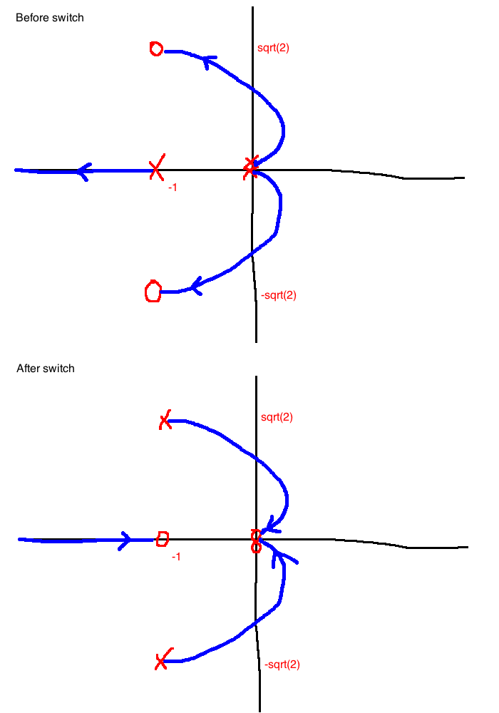
Do the usual root-locus using \(\hat{\pi}(s)=\hat{D}(s)+\hat{K}\hat{N}(s)\). At the end:

1. Turn each X into an O
2. Turn each O into an X
3. Revertse arrows

e.g. 6.3.2

\[\begin{align} P(s)&=\frac{1}{s(s+1)}\\ C(s)&= \frac{s+3}{\tau s+1}\\ \\ \pi(s)&=s(s+1)(\tau s+1)+s+3\\ &= s^2+2s+3+\tau s^2(s+1)\\ \\ \hat{D}(s)&=s^2(s+1)\\ \hat{N}(s)&=s^2+2s+3\\ \hat{K}&=\frac{1}{\tau}\\ \\ \hat{n}&=3, \quad \{0,0,-1\}\\ \hat{m}&=2, \quad \{-1 \pm \sqrt{2}j\}\\ \end{align}\]